Are you wondering how to create an amortization schedule in Excel? Look no further! Mastering the art of building an amortization schedule is a valuable skill for anyone dealing with loans or mortgages. In this step-by-step guide, we will navigate through the intricacies of Excel to simplify the process for you. By the end of this blog, you will be equipped with the knowledge to effortlessly track your loan repayments, interest, and principal amounts. Whether you are a finance professional, a small business owner, or an individual managing personal finances, understanding how to make an amortization schedule in Excel can save you time and provide valuable insights into your financial obligations.
Understanding Amortization and its Significance
Amortization is a financial concept that refers to the spreading out of loan payments over time. It involves the gradual reduction of a debt through regular payments comprising both the principal and interest. By creating an amortization schedule, borrowers can visualize how their loan balance decreases over the repayment period.
Importance of Amortization
Amortization is crucial as it helps borrowers understand how much of their payment goes towards interest and how much reduces the principal owed. This knowledge can assist individuals in making informed financial decisions and planning for the future financial stability.
Benefits of Creating an Amortization Schedule in Excel
By utilizing Excel to create an amortization schedule, individuals can efficiently track their loan progress, experiment with different payment scenarios, and gain insights into potential interest savings. Additionally, Excel provides flexibility in customizing schedules based on specific needs.
Setting Up Your Excel Worksheet
When creating an amortization schedule in Excel, the first step is setting up your worksheet properly to ensure accurate calculations and effective organization. To begin, open a new Excel document and label the columns as follows: Payment Date, Beginning Balance, Payment, Interest, Principal, and Ending Balance. Additionally, include rows for each payment period.
Formatting Cells
To accurately display numerical data, it’s essential to format cells to represent currency values. Select the columns containing monetary figures, navigate to the ‘Number’ tab, and choose the ‘Currency’ option. This step ensures that the payment amounts, interest, and principal values are displayed in the correct format for better readability and analysis.
Setting Formulas
In the ‘Interest’ column, input the formula =B2*$B$1/12 to calculate the interest for each period based on the annual interest rate in cell B1. Next, use the formula =C2-$F$1 in the ‘Principal’ column to determine the portion of the payment that goes towards reducing the loan amount. Finally, update the ‘Ending Balance’ column with the formula =D2-E2 for accurate tracking of the remaining balance after each payment.
Entering Loan Information
When creating an amortization schedule in Excel, the first step is to enter the loan information accurately. Enter the principal amount, interest rate, loan term, and start date in the designated cells. It is crucial to input the correct data to ensure the accuracy of the amortization schedule.
Verify Loan Details
Before proceeding, double-check that the loan details are correct. Ensure the interest rate is in the correct format and the loan term is properly defined.
Organize Data in Excel
To make calculations easier, organize the loan information in a clear format within Excel. Use separate columns for principal, interest rate, monthly payment, and remaining balance.
Calculating Monthly Payments
When creating an amortization schedule in Excel, one crucial step is calculating monthly payments. This calculation helps determine how much a borrower needs to pay each month to gradually reduce the loan balance over time. The formula for calculating monthly payments involves the loan amount, interest rate, and loan term.
Loan Amount and Interest Rate Calculation
In Excel, you can use the PMT function to calculate monthly payments. The formula is =PMT(rate, nper, pv), where rate is the interest rate per period, nper is the total number of periods, and pv is the loan amount. Remember to convert the annual interest rate to a monthly rate for accurate calculations.
You can calculate the monthly interest rate by dividing the annual interest rate by 12. For instance, if the annual interest rate is 6%, the monthly interest rate would be 6%/12 = 0.5%. Plugging in these values into the PMT function will give you the monthly payment amount.
Loan Term and Amortization Schedule
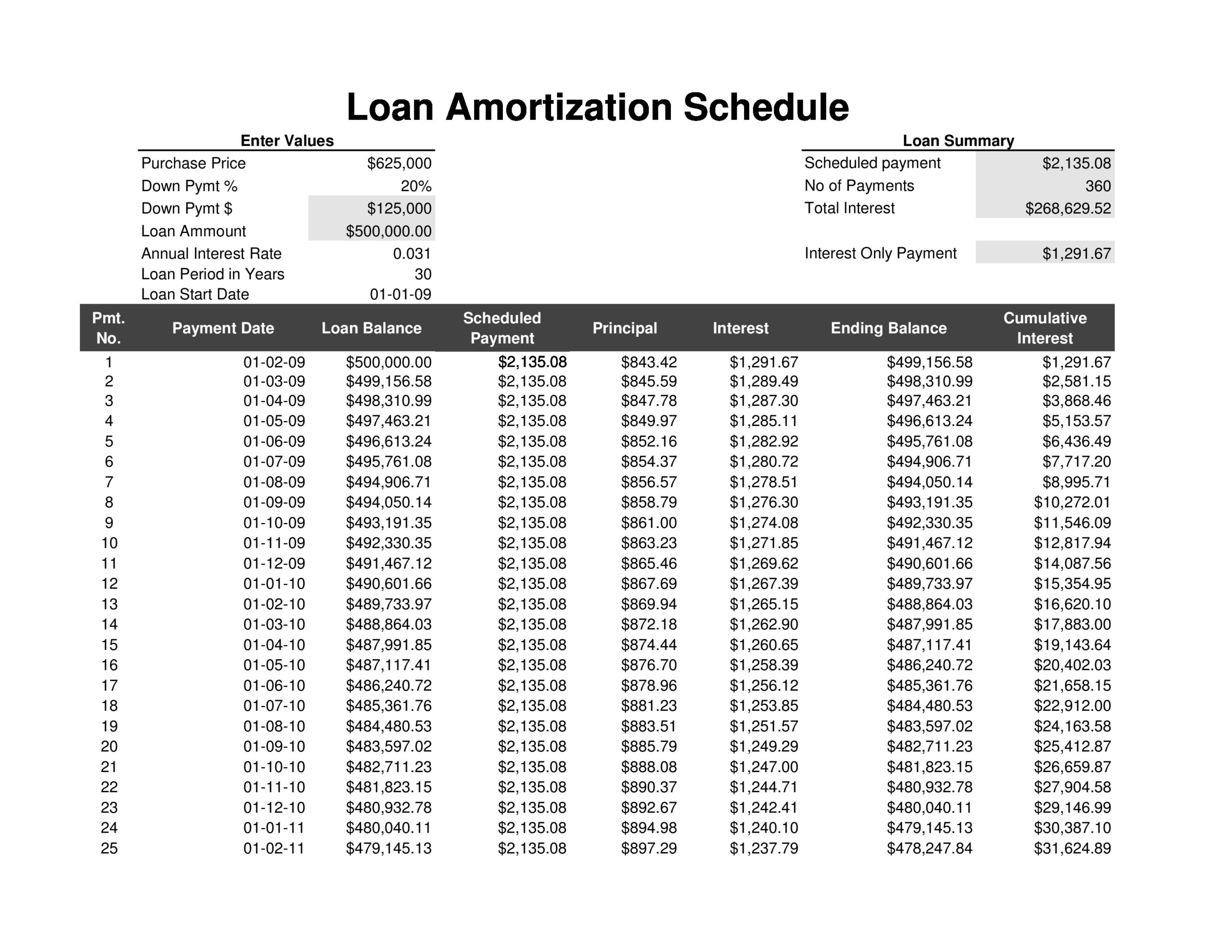
The loan term, usually expressed in years, represents the total number of monthly payments. For example, a 30-year loan has 360 total payments (30 years * 12 months). By inputting the calculated monthly payment, loan amount, and interest rate into Excel, you can create an amortization schedule.
The amortization schedule provides a detailed breakdown of each payment, showing the portion that goes towards principal and interest. This schedule helps borrowers track their progress in paying off the loan and understand how much interest they are paying over time.
Creating the Amortization Schedule Table
When it comes to managing your finances effectively, creating an amortization schedule in Excel can be a valuable tool. By breaking down your loan payments into detailed tables, you can better understand how your payments are allocated towards principal and interest over time.
Setting Up Your Table in Excel
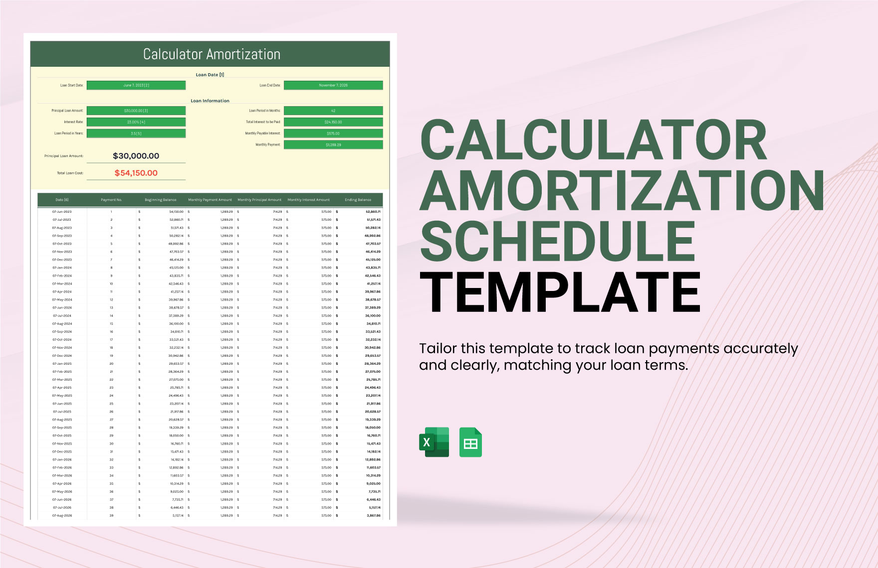
Start by opening Excel and creating a new spreadsheet. Label the columns for payment number, payment amount, principal, interest, and remaining balance. Enter the loan amount, interest rate, and loan term to calculate your monthly payment using the PMT function.
Next, fill in the first row with payment number 1 and populate the corresponding cells with the calculated values. Drag the formula down to fill in subsequent rows, adjusting the remaining balance formula to reflect the decreasing principal.
Customizing Your Amortization Schedule
To enhance the usability of your amortization schedule, consider adding conditional formatting to highlight key information such as when the loan will be paid off or the amount of interest paid over time. You can also insert graphs to visualize the loan repayment progress.
Furthermore, you can add additional columns for extra payments, escrow amounts, or any other relevant details to tailor the table to your specific financial situation.
Customizing the Schedule for Advanced Analysis
When creating an amortization schedule in Excel, the ability to customize the schedule for advanced analysis can provide valuable insights into the loan repayment process. By leveraging Excel’s functionalities, users can tailor the schedule to meet specific requirements and gain a deeper understanding of their financial obligations.
Utilizing Conditional Formatting
One way to enhance the visual appeal of the amortization schedule is by using conditional formatting. This feature allows users to highlight important data points, such as payment due dates or outstanding balances, making it easier to interpret the information at a glance.
Adding Forecasting Capabilities
By incorporating forecasting capabilities into the schedule, users can project future payment amounts based on different scenarios. This feature enables better strategic planning and helps individuals prepare for potential changes in their financial situation.
- Forecasting interest expenses
- Predicting the impact of additional payments
Utilizing Excel Functions for Automation
When creating an amortization schedule in Excel, utilizing Excel functions for automation can significantly streamline the process and ensure accuracy in calculations. To begin, MS Excel offers a range of functions that can be leveraged to automate the calculation of loan repayment schedules, saving time and reducing potential errors.
Utilizing the PMT Function
The PMT function in Excel is a powerful tool for calculating the periodic payment for a loan based on constant payments and a constant interest rate. By inputting the loan amount, interest rate, and number of periods, Excel can automatically generate the payment amount.
Automating the Fill Handle
Excel’s Fill Handle feature allows users to quickly populate a series of cells with a sequence of numbers or formulas. By dragging the Fill Handle, Excel can automatically fill in the remaining cells with the appropriate values, expediting the process of creating an amortization schedule.
Frequently Asked Questions
- What is an amortization schedule?
- An amortization schedule is a table displaying the details of periodic loan payments, including the principal amount, interest amount, and remaining balance.
- Why is creating an amortization schedule in Excel important?
- Creating an amortization schedule in Excel allows you to have a clear overview of how your loan will be repaid over time, helping you understand the payment structure and plan your finances better.
- Can Excel automatically calculate an amortization schedule?
- While Excel does not have a built-in function solely for generating amortization schedules, you can create one using formulas and functions such as PMT, IPMT, PPMT, and others.
- What are the key steps to creating an amortization schedule in Excel?
- The key steps include setting up the necessary columns for the payment schedule, inputting loan details, calculating the monthly payments, and filling in the schedule using formulas.
- How can I customize an amortization schedule in Excel?
- You can customize the schedule by adding additional columns for extra details, changing the formatting for better visual presentation, and adjusting formulas to fit specific loan terms.
Mastering Amortization Schedules in Excel: A Conclusive Guide
Final Thoughts: Creating an amortization schedule in Excel might seem daunting at first, but with the step-by-step guide provided, you can now tackle it with confidence. By following the simple yet detailed process outlined in this blog, you can effectively track your loan payments, understand the interest breakdown, and plan your finances better.
In summary, mastering the art of creating an amortization schedule in Excel empowers you to take control of your financial obligations and make informed decisions regarding loans and investments. Remember, accuracy and consistency are key when setting up your schedule, and with practice, you will become proficient in managing your amortization needs efficiently.
So, dive into Excel, implement the strategies shared, and witness how a well-structured amortization schedule can be a valuable tool in your financial toolkit.