Excel is a powerful tool that can simplify complex financial calculations, such as creating an amortization schedule. If you are looking to master the art of building an amortization schedule in Excel like a pro, you have come to the right place. This blog will walk you through the step-by-step process of setting up an amortization table, calculating principal and interest payments, and ensuring accuracy in your financial projections.

By understanding how to leverage Excel’s functions and formulas effectively, you can streamline the process of generating amortization schedules and gain valuable insights into your loan or mortgage repayments. Let’s dive into the world of financial modeling and learn how to create an amortization schedule in Excel with confidence and precision.
Introduction to Amortization Schedules
Amortization schedules are essential financial tools used to visualize how loans are paid off over time. In the context of Excel, mastering how to create an amortization schedule can empower individuals and businesses to manage their debts efficiently.
Understanding Amortization
Amortization refers to the process of spreading out loan payments over a set period, typically with a fixed interest rate. This ensures that each payment covers both the principal amount borrowed and the interest accrued.
Creating Amortization Schedules in Excel
By leveraging Excel’s functionality, users can easily generate accurate amortization schedules. Using formulas like PMT, IPMT, and PPMT, one can calculate monthly payments, interest portions, and principal repayments.
To start, enter the loan amount, interest rate, loan term, and the start date. Excel can then automate the process of calculating and organizing payment details.
Understanding the Basics of Amortization
Amortization is the process of spreading out a loan into a series of fixed payments over time. In the context of Excel, creating an amortization schedule allows you to see how each payment is allocated between principal and interest. This can be immensely helpful in understanding your loan repayment schedule.
Components of an Amortization Schedule
When you create an amortization schedule in Excel, it typically includes details such as the payment number, payment amount, interest paid, principal paid, and remaining balance. These components help track your progress as you repay your loan.
Calculating Amortization in Excel
To calculate amortization in Excel, you can use built-in functions like PMT, PPMT, and IPMT. These functions help determine the total payment, principal payment, and interest payment for each period. By utilizing these functions, you can easily create an accurate amortization schedule.
Setting Up Your Excel Spreadsheet
When creating an amortization schedule in Excel, the first step is to set up your spreadsheet properly to ensure accurate calculations. Start by opening a new Excel workbook and labeling the necessary columns: Loan Amount, Interest Rate, Number of Payments, Payment Amount, Loan Start Date, and Remaining Balance.
Inserting Formulas
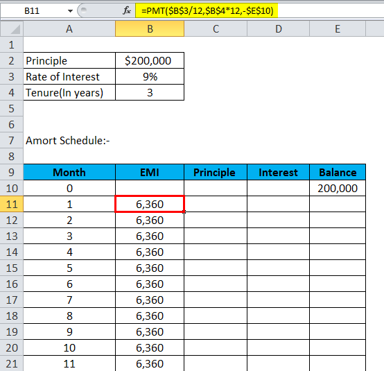
Next, insert the appropriate formulas to calculate the monthly payment based on the loan amount, interest rate, and number of payments. You can use the PMT function in Excel to simplify this calculation. =PMT(rate, nper, pv)
For example, if your loan amount is $100,000, interest rate is 5%, and the loan term is 5 years with monthly payments, the formula would look like this: =PMT(5%/12, 5*12, 100000).
Formatting Cells
Once you have inserted the formulas, format the cells to display currency values correctly. Select the cells containing the payment amount, loan amount, and remaining balance, and apply the currency format to ensure clarity.
Additionally, format the loan start date column as a Date field to track the payment schedule accurately.
Calculating Monthly Payments
Calculating monthly payments is a crucial step in creating an amortization schedule in Excel. To determine the monthly payment, you can use the PMT function, which helps in calculating the total payment made over a loan’s life.
Using the PMT Function
To use the PMT function in Excel, you need to enter the formula in a cell: =PMT(rate, nper, pv). Here, the rate represents the interest rate per period, nper is the total number of payment periods, and pv stands for the present value or loan amount.
Interpreting the Result
The result you get from the PMT function represents the fixed monthly payment needed to pay off the loan in full. This amount includes both the principal and interest, ensuring a consistent payment throughout the loan term.
Creating the Amortization Schedule Table
When it comes to managing financial records and planning future payments efficiently, having an amortization schedule is essential. Using Excel, you can easily create a detailed amortization schedule that breaks down each payment into principal and interest components.
Setting Up the Table
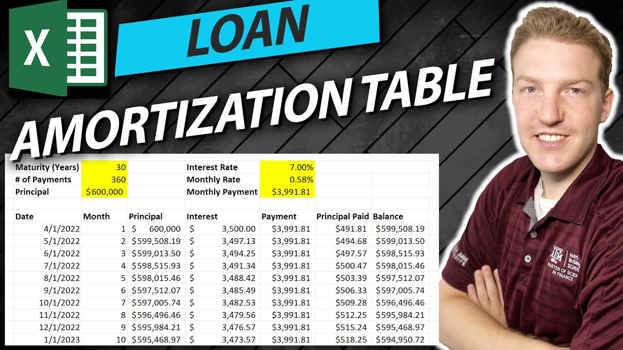
Start by opening a new Excel spreadsheet and labeling columns for Payment Number, Payment Amount, Principal, Interest, and Remaining Balance. Make sure to include the necessary calculations for each column.
Filling in Payment Details
Enter the loan amount, interest rate, and loan term to calculate the monthly payment. Use Excel formulas like PMT to determine the payment amount. Then, fill in the principal and interest amounts for each payment.
- Principal: The portion of the payment that goes towards reducing the loan balance.
- Interest: The cost of borrowing, calculated based on the remaining balance and interest rate.
Adding Extra Payments
When creating an amortization schedule in Excel, you may want to explore the impact of making extra payments on your loan. By incorporating additional payments towards the principal, you can save on interest and pay off your loan faster.
Calculating Extra Payments
To determine the effect of extra payments on your loan, you can utilize the PMT function in Excel. This function helps calculate the new monthly payment after making additional payments towards the principal amount. Use the formula: =PMT(rate,nper,-(pv+extra payment),fv), where the extra payment is the amount you wish to pay in addition to your regular monthly installment.
Tracking Progress with a Chart
Visualizing the impact of extra payments can be done effectively using a chart in Excel. Create a line graph showing the decreasing loan balance over time as extra payments are made. This graphical representation can motivate you to continue making additional payments and accelerate your debt payoff journey.
Visualizing Data with Charts
When working with amortization schedules in Excel, creating charts can help in visualizing the data more effectively. Charts can provide a clear representation of the loan repayment schedule over time, making it easier to analyze and understand the data.
Types of Charts to Use
Excel offers various types of charts that can be used to represent amortization schedules. Line charts, column charts, and pie charts are commonly used to visualize data related to loan payments and interest calculations. Each type of chart has its unique advantages in presenting the information.
You can use a line chart to track the decreasing loan balance over the payment period, a column chart to compare different payment components, or a pie chart to show the proportion of interest and principal payments.
Creating Charts in Excel
To create a chart in Excel, select the data you want to include in the chart, go to the “Insert” tab, and choose the type of chart you want to create. You can customize the chart by adding titles, labels, and legends to make it more informative and visually appealing.
Pro tip: Use the chart tools in Excel to modify colors, styles, and layouts to enhance the visual representation of your amortization schedule.
Frequently Asked Questions
- What is an amortization schedule?
- An amortization schedule is a table that shows the breakdown of loan payments into interest and principal amounts over the life of a loan.
- Why is it important to create an amortization schedule?
- Creating an amortization schedule helps borrowers understand how much of each loan payment goes towards interest and how much goes towards reducing the principal balance. It also provides a clear overview of the total cost of the loan.
- How can Excel help in creating an amortization schedule?
- Excel provides powerful tools and functions that make it easy to set up formulas to calculate loan amortization. It allows users to customize the schedule based on different parameters such as loan amount, interest rate, and loan term.
- What key Excel functions are useful for creating an amortization schedule?
- Functions like PMT, IPMT, PPMT, and FV in Excel are commonly used to calculate loan payment amounts, interest payments, principal payments, and remaining balances, respectively, when creating an amortization schedule.
- Is there a step-by-step guide to creating an amortization schedule in Excel?
- Yes, the blog post provides a detailed step-by-step guide on how to create an amortization schedule in Excel like a pro. It covers setting up the data, inputting formulas, and formatting the schedule for easy readability.
Unlock Your Excel Skills with Amortization Schedule Mastery
Creating an amortization schedule in Excel may seem daunting at first, but with the right guidance and tools, you can tackle it like a pro. By following the steps outlined in this blog, you now possess the knowledge to efficiently structure your loan repayments and understand your financial obligations better.
Remember, attention to detail and consistency are key when mastering Excel functions. Practice regularly to enhance your skills and stay updated with the latest features in Excel. Whether you are a finance professional or a student, mastering the art of creating amortization schedules will not only save you time but also elevate your spreadsheet proficiency to new heights.
So, dive into your Excel sheets with confidence, unleash your creativity, and let your amortization schedules reflect your expertise. Excel at Excel, and excel in your financial management endeavors!