Are you looking to gain mastery in creating an amortization schedule in Excel? Understanding how to make an amortization schedule in Excel is a valuable skill for anyone managing loans or investments. By breaking down complex financial calculations into manageable steps, you can effectively track payments and interest over time. In our step-by-step guide, we will delve into the intricacies of building an accurate and efficient amortization schedule using Excel. Whether you are a finance professional, a student, or a curious individual wanting to enhance your Excel skills, this tutorial will equip you with the knowledge to create precise loan repayment schedules with ease.

Introduction to Amortization Schedules
An amortization schedule is a table that shows the periodic payments on a loan or mortgage, breaking down the principal and interest components. In Excel, creating an amortization schedule provides a clear picture of how the loan balance decreases over time.
Understanding Amortization
Amortization is the process of paying off a debt over time through regular payments. Each payment covers both the interest on the outstanding balance and a portion of the principal amount.
Interest vs. Principal
Interest is the cost of borrowing money, while the principal is the original loan amount. As payments are made, the interest portion decreases, and the principal repayment increases.
Understanding the Importance of Amortization Schedules
Amortization schedules play a crucial role in financial planning, especially when dealing with loans or mortgages. They provide a detailed breakdown of how each payment is allocated towards principal and interest over the term of the loan.
The Structure of an Amortization Schedule
An amortization schedule typically consists of columns that show the payment number, payment amount, interest paid, principal paid, and remaining balance.
These schedules help borrowers understand how much of each payment goes towards reducing the loan balance and how much goes towards interest.
Tracking Loan Repayment Progress
By following an amortization schedule, individuals can track their progress in repaying the loan.
This helps in budgeting and planning for future payments, ensuring that each payment contributes to reducing the total amount owed.
Gathering Data for Your Amortization Schedule
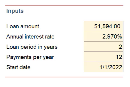
When creating an amortization schedule in Excel, the first step is to gather all the necessary data. Start by collecting the loan amount, interest rate, loan term, and payment frequency.
Loan Amount and Interest Rate
Enter the initial loan amount and the annual interest rate into your Excel spreadsheet. Make sure to format the cells correctly to reflect currency and percentage values. This step is crucial for accurate calculations.
Loan Term and Payment Frequency
Specify the loan term in years and the payment frequency (monthly, quarterly, etc.). This information will help you determine the number of payments and the payment amount per period. Ensure to use consistent units throughout.
- For monthly payments, divide the annual interest rate by 12.
- For quarterly payments, divide the annual interest rate by 4.
Setting Up Your Excel Spreadsheet
When creating an amortization schedule in Excel, the first step is setting up your spreadsheet. Start by inputting the necessary information in separate columns to organize your data efficiently.
Column Setup
Create columns for elements like loan amount, interest rate, loan term, payment frequency, payment date, principal paid, interest paid, and remaining balance. Use headings and labels to clearly indicate the purpose of each column.
Data Entry
Enter the loan details accurately in their respective columns. Make sure to include formulas for calculating interest, principal, and remaining balance based on the payment schedule.
Formatting Cells
Apply proper cell formatting, such as date formats for payment dates and currency formats for monetary values. Use conditional formatting to highlight important data points, like overdue payments or loan completion.
Calculating Monthly Payments
When creating an amortization schedule in Excel, one of the key components is calculating the monthly payments. To do this, you need to consider the loan amount, interest rate, and loan term.
Determining Loan Amount
Begin by entering the loan amount into the designated cell. This is the total amount of money borrowed.
Input the interest rate: 5% Annual Interest
Enter the loan term: 30 Year Loan
Calculating Monthly Payments
To calculate monthly payments, use the formula: =(PMT(interest rate/12, loan term*12, loan amount))
- Divide the annual interest rate by 12 to get the monthly interest rate.
- Multiply the loan term by 12 to convert years into months.
- Use the PMT function to find the monthly payment amount.
Creating the Amortization Table
When creating an amortization table in Excel, it’s essential to follow a step-by-step approach to ensure accuracy in repayment calculations.
Setting Up the Table
To start, create columns for payment number, payment amount, principal paid, interest paid, and remaining balance. Use proper formulas to calculate these values accurately.
It’s crucial to ensure that your formulas are correctly referencing the loan amount, interest rate, and loan term to provide accurate results. Be meticulous in inputting the data.
Populating the Table
Once the table layout is set up, manually input the initial loan amount, interest rate, and loan term. Excel will then help populate the remaining columns using the calculated values based on your input.
- Enter the loan amount in the principal column.
- Calculate the monthly interest by multiplying the remaining balance by the monthly interest rate.
- Subtract the interest from the total monthly payment to determine the principal repayment amount.
- Repeat the process for each month until the remaining balance reaches zero.
Visualizing Your Amortization Schedule
When creating an amortization schedule in Excel, it’s essential to visualize the data for a better understanding of how your payments are distributed over time.
Creating a Line Chart
To visualize your amortization schedule, you can create a line chart that illustrates the principal and interest payments over the loan term.
You can utilize Excel’s chart tools to plot the data points and connect them to see the trend clearly.
Customizing the Chart
Customize the chart by adding axis labels, titles, and legends to make it more informative.
- Use different colors for principal and interest payments for easy identification.
- Include a trendline to visualize the overall loan repayment trajectory.
Customizing Your Amortization Schedule
When creating an amortization schedule in Excel, you can further customize it to meet your specific needs. Whether you want to adjust payment frequencies, include extra payments, or visualize data differently, Excel offers a range of tools to help you tailor your schedule.
Payment Frequency Adjustment
If you wish to change the frequency of your payments, Excel allows you to easily adjust this aspect. By modifying the formula used to calculate payments, you can switch between monthly, bi-weekly, quarterly, or even annual payment schedules.
You can use Excel functions like PMTPRINC and PMT to calculate payments based on different frequencies while keeping the schedule accurate.
Adding Extra Payments
Want to see how making extra payments can impact your loan repayment? Excel enables you to incorporate additional payments into your amortization schedule. By inserting the extra payment amounts into the respective periods, you can observe the revised payoff timeline.
Here you can utilize the IF function to account for the extra payments effectively within your schedule.
Data Visualization Techniques
Visual representation of amortization data can provide a clearer understanding of your loan terms. Excel offers charting tools that allow you to create graphs or charts to represent payment schedules, interest breakdowns, or loan balances over time.
Consider using Excel’s Line Chart or Pie Chart features to present your amortization details visually for better analysis and decision-making.
Advanced Tips and Tricks
Enhance your amortization schedule in Excel with these advanced tips and tricks to optimize your financial planning process.
Utilize Conditional Formatting
Highlight important information using conditional formatting to make it stand out for better visibility.
Customize cell colors based on specific criteria to emphasize key data.
Implement Data Validation
Ensure data accuracy by setting data validation rules that restrict entries to a certain format or range.
- Create drop-down menus for consistent input.
- Restrict dates, numbers, or text to prevent errors.
Frequently Asked Questions
- What is an amortization schedule?
- An amortization schedule is a table displaying the breakdown of loan payments into interest and principal over the life of a loan. It shows how each payment is allocated between reducing the balance and paying interest.
- Why is it important to create an amortization schedule in Excel?
- Creating an amortization schedule in Excel allows you to visually understand how your loan payments are structured, track your progress in paying off the loan, and make informed financial decisions.
- What are the key steps to creating an amortization schedule in Excel?
- The key steps include setting up the necessary columns, inputting the loan details, calculating the monthly payment, and using Excel formulas to determine the interest and principal portions of each payment.
- Can Excel automatically generate an amortization schedule?
- While Excel doesn’t have a built-in function specifically for creating an amortization schedule, you can use formulas like PMT, IPMT, and PPMT to calculate the payment amount, interest portion, and principal portion for each period.
- How can I customize an amortization schedule in Excel?
- You can customize the schedule by adding extra columns for additional calculations, changing the payment frequency, adjusting the payment amounts, or incorporating extra payments to see their impact on the loan term.
Unlocking Excel’s Power: Concluding the Amortization Schedule Mastery
As we conclude our journey on how to make an amortization schedule in Excel, it’s clear that mastering this financial tool can have a significant impact on your financial planning and decision-making. By following the step-by-step guide provided, you can now confidently create accurate amortization schedules to manage your loans effectively.
Remember, the key takeaways include understanding the formulae involved, utilizing Excel’s functions efficiently, and paying attention to detail to avoid errors. By incorporating these principles into your financial repertoire, you can navigate loan repayments with ease and precision.
Excel’s versatility knows no bounds, and by honing your skills in creating amortization schedules, you are unlocking a powerful tool for financial success. So, go ahead, practice, and perfect your craft to empower your financial journey!